OEE From First Principles
Find the Real Opportunity in Your Process
Most operations teams have some picture of equipment performance. Shift reports, OEE dashboards, downtime logs. The problem is not that the data does not exist. The problem is that the picture is rarely complete, and an incomplete picture can be more dangerous than no picture at all.
A partial view of performance can make a line look healthy when it is not. It can point improvement effort at the wrong step. It can justify inaction when action is needed. It can hide the real constraint behind a number that looks acceptable on a dashboard but does not reflect what the process is actually capable of.
This diagnostic is about building a complete picture, step by step, in a single unit that everyone agrees on, so that the signals you act on are the right ones.
Work through the six steps in order. Each one builds on the last.
- Step 1 — Define Your Process Boundaries — Map the material flow and identify each piece of equipment in sequence
- Step 2 — Agree the Common Throughput Unit — Establish the single unit everything converts to, and understand where the bottleneck really is
- Step 3 — Determine the Equipment Rates — Engineering, qualified, best demonstrated performance, and average for each step
- Step 4 — Calculate OEE — Availability, performance, and quality, step by step, with throughput alongside the percentage
- Step 5 — Build the Picture — Make the gap visible and identify the true constraints (performance and qualified)
- Step 6 — Detail Your Loss Categories — Build a complete picture of where the opportunities lie and what each one is worth
Do not skip ahead. The picture in Step 5 is only as good as the work you do in Steps 1 and 2.
Key Definitions:
- Throughput — output rate in a common unit (e.g. kg finished goods / day). Always stated with a time period.
- Capacity — the maximum sustainable throughput under defined conditions. This diagnostic uses four levels: Engineering, Qualified, Best Demonstrated, and Average.
- Overall Equipment Effectiveness — Availability × Performance × Quality. The % of good product made vs. the total potential product made on the same equipment in the same time.
Step 1 — Define Your Process Boundaries
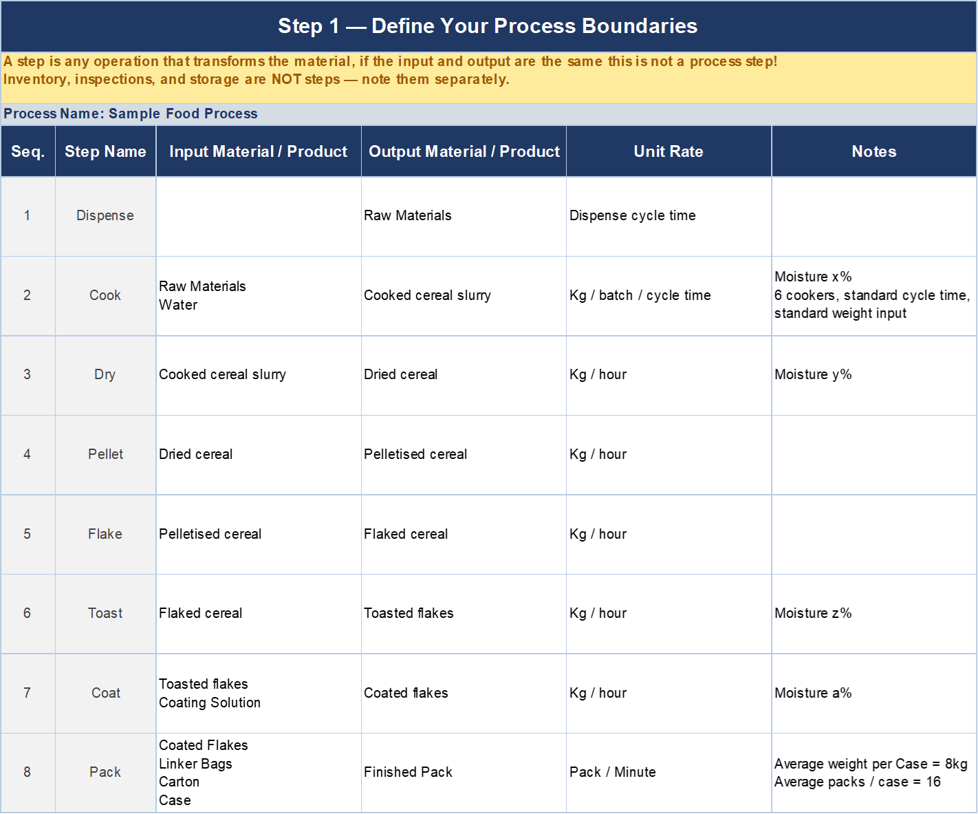
A step is any operation that transforms the material, in form, state, composition, or condition. Blending is a step. Granulation is a step. Drying is a step. Filling is a step. Labelling is a step.
Inventory between operations is not a step. It is a signal. If you have significant inventory sitting between two steps, note it on your map, but do not treat it as a step. It may show up later in Step 6 as a scheduling or flow loss.
A simple test: Does this operation change what the material is, or what it looks like? If yes, it is a step. If it only changes where the material is, or how long it has been waiting, it is not. If the input and the output of an operation are the same material in the same state, it is not a step.
By the end of Step 1 you will have, for each step in your process:
- What goes in — All materials (raw, pack, prior step outputs/WIP, water, etc.)
- What comes out — Transformed material in whatever form or state it leaves that step, any waste materials
- The sequence — The order the steps connect, from the start of the process to the finished output
- A unit rate for each step — Even a rough one. You will refine it in Step 3, but noting it now flags immediately where batch steps and continuous steps sit alongside each other. That difference matters in Step 2.
Keep it simple. This is a material flow map to identify equipment performance step by step, not a value stream map, not a process specification. The purpose is to know what equipment is doing what, in sequence, so you can measure each one. If you can draw it on one page, you have done it right.
Step 2 — Agree the Common Throughput Unit
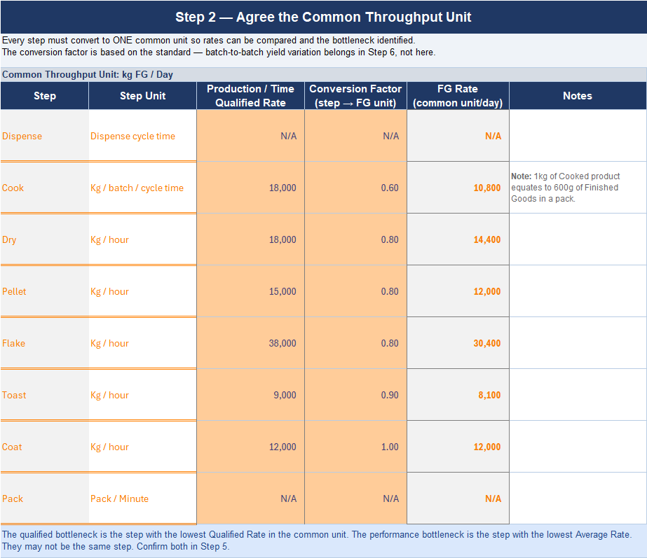
Before you can compare performance across steps, every step in your process must be expressed in the same unit. This is the common throughput unit. You will use it for every rate, every chart, and every comparison from this point forward.
For most finished goods operations this will be finished pack or kg of finished goods. That is the unit everything else converts back to.
Intermediate steps are where it gets complicated. A blending step works in kg of blend. A granulation step works in kg of granulate. A filling step works in units filled. Each of these is a different unit, but each one produces something that eventually becomes a finished pack. The conversion factor is what connects them.
For each step, record 3 things:
- The step unit (what the equipment measures — kg/batch, kg/hour, packs/minute)
- The qualified rate in that step unit
- The conversion factor to the common unit
Write it down. Agree it as a team. If anyone disagrees with a conversion factor, resolve it now, not after you have built the chart.
Note: The FG Rate = Qualified Rate × Conversion Factor. This is the number that goes into every comparison from here forward.
Note: Batch steps and continuous steps cannot be compared until they are in the same unit. A cook step running in kg per batch per cycle time and a dryer running kg per hour are not directly comparable.
Important: batch-to-batch variation in yield is not a reason to change the conversion factor. Yield variation is a process loss. It belongs in Step 6. The conversion factor is based on the standard, what one unit of input at this step should produce under normal conditions.
Understanding where the bottleneck really is:
This is also the step where you begin to see something important. Improving OEE on one piece of equipment does not automatically improve the throughput of the line. It only improves line throughput if that equipment is the bottleneck. And there are two types of bottleneck worth understanding now, before you go any further.
- The qualified bottleneck — The step with the lowest qualified rate in the common unit. This is the structural qualified ceiling of the line as it is currently validated. No amount of improvement work changes this without a revalidation project.
- The performance bottleneck — The step with the lowest average rate in the common unit. This is where the line is actually being constrained today. It may be the same step as the qualified bottleneck, or it may not.
Knowing which is which changes where you focus. You will confirm both when you build the picture in Step 5. But the common throughput unit is what makes that comparison possible.
Step 3 — Determine the Equipment Rates for Each Step
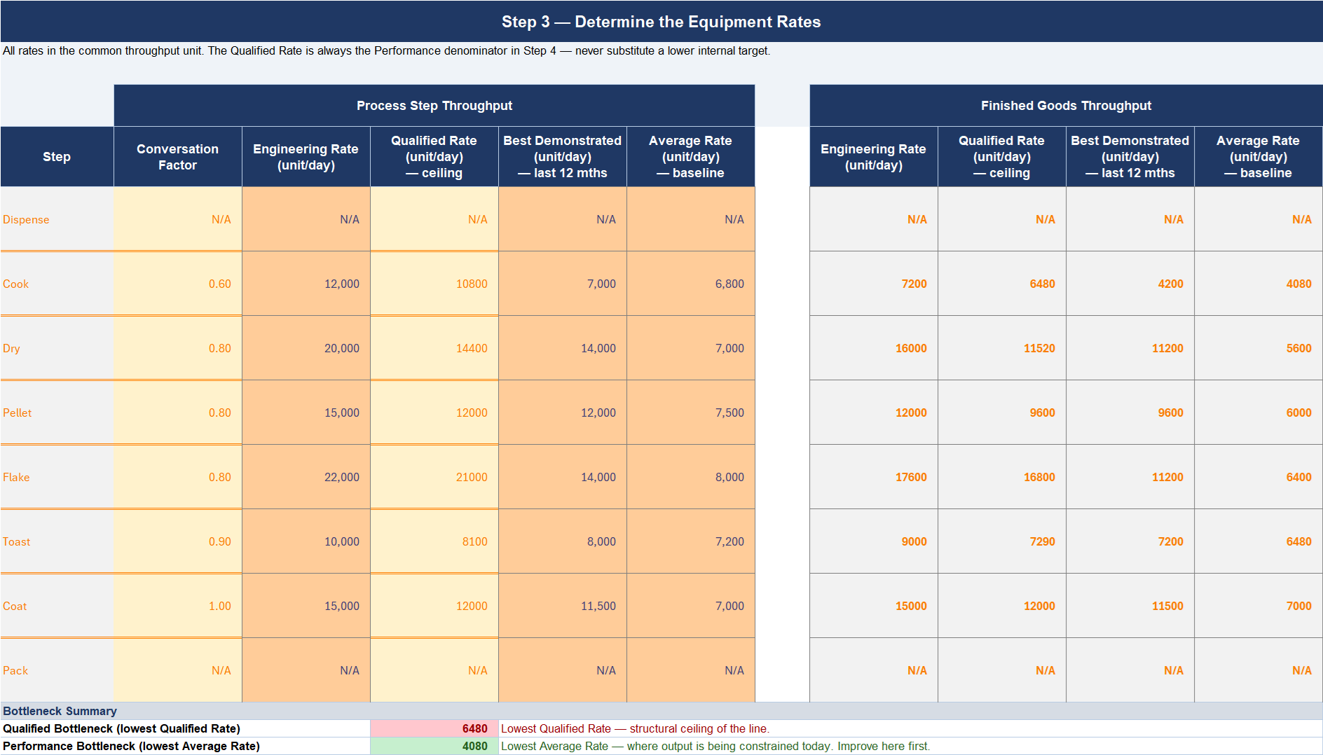
This is where you establish the four rates for each step. All rates must be expressed in the common throughput unit agreed in Step 2. If a rate is not in that unit, convert it before you record it.
Engineering Rate
What the equipment was designed and built to do. This is the manufacturer's specification, the theoretical ceiling. It assumes perfect conditions, no variation, no process constraints. It is rarely achievable in practice, but it sets the upper bound of what the equipment is capable of.
Qualified Rate
The rate the line was validated at. In regulated environments this is the rate formally demonstrated, documented, and approved. You cannot run faster than this without revalidation. It is the operational ceiling, the fastest you are allowed to run.
For batch processes, express this as: validated batch size \ validated cycle time, converted to your common throughput unit per time.
Best Demonstrated Rate
The best the line has actually demonstrated over the past 12 months. This is not an average, it is the best sustained output achieved under normal operating conditions. Use an appropriate length depending on your process cycle times to ensure it includes standard conditions such as changeovers and maintenance. This filters out single-shift spikes and reflects what is genuinely repeatable today, without any capital investment or revalidation.
Average Rate
What the line actually produces on a typical day, averaged across the same window. This is your baseline. Everything above it is opportunity.
Step 4 — Calculate OEE for Each Step
For each step, calculate OEE from first principles using three components.
Availability — The proportion of planned production time during which the step was actually running.
Performance — How close to the qualified rate the step ran when it was running. This includes minor stoppages and idling times. The qualified rate is always the denominator here.
Quality — The proportion of output that met specification first time, without rework or rejection.
OEE = Availability * Performance * Quality
Express the result as a percentage. Actual performance throughput for each step is also your Average rate in common throughput unit per time. The OEE percentage tells you the efficiency. The throughput number tells you the impact. You need both.
A step running at 65% OEE on a line with a qualified rate of 1,000 Kg per day is losing 350 Kg per day. That is the number that connects to revenue. The percentage alone does not.
Do this for every step individually. Do not aggregate across steps yet, you need to see each step on its own first.
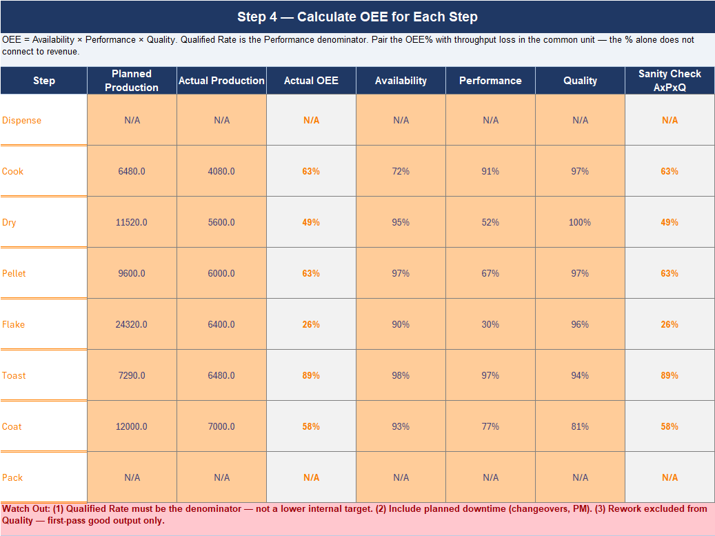
Watch out: OEE is easy to inflate. The three most common ways are
- Using a rate lower than the qualified rate as the performance denominator
- Excluding planned downtime that should be included
- Omitting rework from the quality calculation.
If your OEE looks better than you expected, check these three things first.
Step 5 — Build the Picture by Step
This is where the diagnostic becomes visible. For each step, build a stacked bar in the common throughput unit. The bar shows all four rates as bands, stacked from the bottom up.
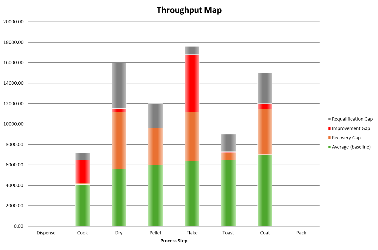
Each band has a different owner and a different cost to close.
- Recovery Opportunity (gap from Average to Best Demonstrated): performance you have already demonstrated. No capital, no revalidation. This is the first conversation.
- Improvement Opportunity (gap from Best Demonstrated to Qualified): process stability work. Requires investigation and sustained effort, but no regulatory submission.
- Requalification Opportunity (gap from Qualified to Engineering): requires a formal validation project. A different budget cycle entirely.
Place the bars for every step side by side. Two things will become clear immediately.
First, the constraint. The constraint is the step with the lowest throughput in the common unit. Everything else in the process is secondary to that step until it is resolved. Improving any other step first is effort spent in the wrong place. You will also now be able to confirm whether the qualified bottleneck and the performance bottleneck are the same step, or whether the line is being constrained today by something other than its structural ceiling.
Second, the nature of the gap. A process where most of the gap sits in the Recovery Opportunity band has a consistency problem. A process where most of the gap sits in the Improvement Opportunity band has a process stability problem. A process where the Qualified Rate is far below the Engineering Rate has a revalidation conversation waiting to happen.
None of those matter if the improvement just moves the bottleneck slightly, a comprehensive improvement plan is needed end to end.
Step 6 — Define Your Loss Categories
Now you know the size of the gap. This step is about understanding what is specifically causing it, and building a picture of where your opportunities lie, who owns each one, and what each one is worth.
For each identified, impactful, step, categorise the losses that explain the difference between your Average Rate and your Qualified Rate. Start with unplanned losses. These are the losses you can act on immediately, without a capital project or a regulatory submission.
Unplanned downtime — Breakdowns, faults, waiting for materials, waiting for people, waiting for decisions. These are the stops that were not planned and should not have happened.
Minor stops — Short unplanned stoppages that individually seem insignificant but collectively represent a large loss. Often undercounted because they are not deliberately logged. A line that stops for two minutes, twenty times a shift, has lost forty minutes of production that rarely appears as its own category in any report.
Speed loss — Running below the qualified rate when the line is running. This is often invisible because the line appears to be working. It is not working at the rate it should be.
Quality loss — Defects, rework, and first-pass failures. Include rework even if the material is eventually recovered, the time and resource spent is still a loss.
Planned downtime — Changeovers and planned maintenance. These are real losses in throughput terms, even if they are necessary. Understanding their true cost in the common throughput unit often changes the conversation about changeover frequency and maintenance scheduling.
Unplanned no-run time — The line was not scheduled to run, but not for a planned reason. Demand shortfall, material unavailability, scheduling gaps. This is important to separate from planned downtime. It is not an equipment problem. It is a planning and scheduling problem, and it belongs in a different conversation. Note: This category sits outside OEE as standardly defined. It is included here because it is commonly mistaken for an equipment loss, knowing it is a scheduling problem prevents the wrong team from being assigned to fix it.
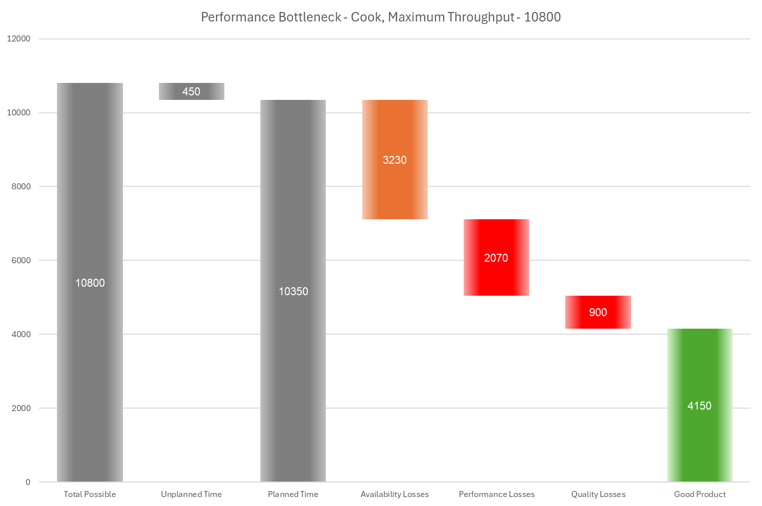
For each loss category:
Quantify it in the common throughput unit. A loss that cannot be quantified cannot be prioritised. The waterfall from Qualified Rate down to Average Rate, with each loss category as a bar, is your business case. It shows exactly where the opportunity sits, what it would be worth to close each gap, and who needs to own the work to close it.
The purpose of this step is not to arrive at a number. It is to build a picture, complete enough that the right people can see the right opportunities and make the right decisions about where to act first.
What This Tells You
By the end of Step 6 you have two things.
Key Links:
The tools section includes a OEE and Throughput Diagnostic Tool in excel to help you determine your rates, conversion factors , and associated opportunities.
 Damon Reid